AI CERTS
4 hours ago
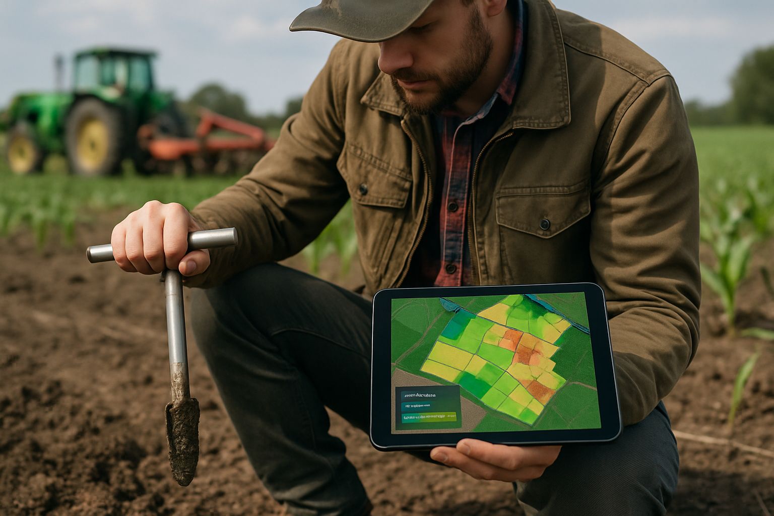
Quantile regression forests sharpen soil uncertainty mapping
Consequently, users receive spatial layers showing estimated medians plus low and high bounds. Farm planners can then rank fields by risk, dosage, and return. Meanwhile, ML engineers appreciate that the algorithm scales to millions of sensing driven covariate stacks. This article unpacks the data need, the mechanics, recent benchmarks, and practical deployment steps. It closes with emerging research and training resources.
Mapping Needs And Gaps
Digital soil programs face pressing accuracy expectations from carbon markets and nutrient regulators. Moreover, remote sensing delivers terabytes of predictors yet hides heterogeneity below the plow layer. Standard regression yields one value per pixel. In contrast, land stewards want a spread that reflects sampling density and terrain complexity. Risk savvy agriculture investors therefore ask for calibrated intervals before committing fertilizer budgets. Consequently, uncertainty communication has become an operational KPI for soil agencies. Policies now cite PICP and CRPS thresholds alongside R² targets. These drivers frame the search for robust distributional algorithms. Stakeholders need pixel wise spreads, not single values. The next section clarifies how Quantile regression forests meet that demand.
Quantile regression forests explained
Quantile regression forests extend Breiman's random forests by storing full outcome lists inside terminal nodes. Specifically, each tree votes with a weight proportional to proximity in covariate space. The ensemble then forms an empirical cumulative distribution for any requested location. Consequently, percentiles such as the fifth and ninety-fifth emerge without parametric assumptions. Users simply read the desired quantile to build a prediction interval. Meanwhile, computational cost stays close to classic random forest inference. That scalability attracts ML teams handling massive remote sensing mosaics. Nevertheless, the algorithm cannot predict beyond the training range of soil properties. QRF thus couples flexibility with distribution outputs at negligible additional compute. Real world soil mapping now demonstrates those advantages.
Operational Soil Mapping Examples
Moreover, public datasets showcase the algorithm at continental scale. SoilGrids 2.0 publishes median, lower, and upper bounds for six depths using ranger software. Consequently, global planners access 90% intervals for carbon accounting.
- Australia mapped 90,025 samples with Quantile regression forests and achieved nominal 90% coverage.
- Andhra Pradesh study reported PICP 90.2% for soil depth intervals.
- Chilean forestry mapping reached SOM R² 0.61 using the same approach.
Meanwhile, each project validated prediction intervals with withheld observations. Nevertheless, reported coverage sometimes deviated in sparsely sampled highlands. Teams flagged those tiles to caution agriculture advisors working there. These examples confirm scalable performance and highlight calibration duties. The following section weighs strengths against known limits.
Strengths And Known Limits
Firstly, the approach handles mixed numeric and categorical covariates without transformation. Therefore, analysts merge terrain, climate, and satellite layers effortlessly. Secondly, bagging delivers stable performance even when ML engineers add hundreds of inputs. In contrast, Gaussian processes struggle beyond several thousand samples. Quantile regression forests also output intervals bounded within observed soil properties. Nevertheless, that bound prevents extrapolation into unmeasured extreme salinity or peat depths. Furthermore, coverage may drift when covariate combinations depart from training density. Users must therefore compute PICP, CRPS, and pinball loss during validation. Strengths outweigh limits for routine mapping, yet diligence remains essential. Alternatives and hybrids can mitigate the listed weaknesses.
Alternatives And Hybrid Methods
Moreover, recent studies apply distribution-free conformal prediction on top of tree ensembles. The Monte Carlo variant delivered 91% empirical uncertainty coverage for spectral CNNs with reduced interval width. Consequently, some teams wrap Quantile regression forests with conformal calibration to guarantee nominal rates. Bayesian neural networks and MC dropout tackle parameter risk but often yield wider bands. Nevertheless, they scale poorly when thousands of sensing tiles arrive daily. Gaussian processes still excel at smaller sites requiring full covariance but cannot cover continental agriculture layers. Therefore, many operators stick with Quantile regression forests while experimenting with lightweight calibrators. Hybrid stacks thus balance speed and statistical reliability. Implementation details decide whether those gains materialize.
Practical Implementation Best Practices
Practitioners must tune forests before pushing models into production. Firstly, set Quantile regression forests tree counts above 500 to stabilize tail quantiles. Then, select the conditional forest weighting option or Greenwald-Khanna summaries for memory efficiency. Meanwhile, compute prediction interval coverage on a spatially stratified validation set to track uncertainty. Log pinball loss across each soil depth to compare properties fairness. Additionally, integrate ML metadata logging in reproducible notebooks for auditing by stakeholders. Professionals can deepen expertise with the AI Learning Development™ certification. Consequently, teams align model governance with recognized industry standards. Attentive tuning and documentation secure reproducible, transparent results. Future research will further streamline these routines.
Future Directions And Research
Looking ahead, hardware advances will shorten training times for global stacks. Moreover, coverforest promises drop-in conformal calibration borrowed from online learning theory. Consequently, Quantile regression forests could gain guaranteed coverage without extra ensembles. AutoML pipelines already test competing ML regressors and select the best interval width. Nevertheless, researchers still need standardized uncertainty dashboards for stakeholder communication. Future benchmarks will compare soil properties calibration across biomes, depths, and temporal windows. Therefore, collaborations between earth observation firms and agriculture ministries will intensify. Continued community standards will keep predictive maps honest and actionable. The conclusion recaps central insights and invites further skill building.
Soil stewards no longer settle for single best guesses. Instead, the techniques presented here deliver credible distribution maps at operational scale. QRF paired with diligent validation already drives site-specific agriculture advice and carbon reporting. Meanwhile, conformal methods and AutoML promise tighter bands without extra complexity. Successful teams track coverage metrics, document settings, and retrain when new sensing layers arrive. Additionally, continuous learning keeps staff aligned with evolving standards. Readers seeking structured growth can enroll in the AI Learning Development™ program. Apply the practices discussed today and turn soil data into confident, timely decisions.


